6.036 Project 2: MNIST Classifiers
This project is about digit classification using the MNIST database. It contains 60,000 training digits and 10,000 testing digits. The goal is to practically explore differenet classifiers and evaluate their performances. The exploration ranges from simplest classifier, e.g.,linear regression with softmax for classification, to deep nerual networks.
This report will be available online after due date at: http://kehang.github.io/
for people (including graders) to review. After grading, the post will be modified to be a standalone report with more background.
Package specifications for this project:
-
OS: Mac
-
python: 3.6.0
-
keras: 2.0.2
-
backend of keras: theano
-
theano: 0.9.0
1. Multinomial/Softmax Regression
Part 4: report base-line test error
when temperature parameter = 1, the test error is 0.1005, implying the linear softmax regression model is able to recognize MNIST digits with around 90%.
Part 5: explain temperate parameter effects
Increasing temperature parameter would decrease the probability of a sample \(x^{(i)}\) being assigned a label that has a large \(\theta\), and increase for labels with small \(\theta\). The mathematic explanation is following:
\[P_j = \frac{exp(\theta_j x / \tau)}{\sum_k exp(\theta_k x / \tau)}\] \[\frac{\partial log(P_j)}{\partial \tau} = \frac{1}{\tau^2} \Big[ \frac{\sum_k exp(\theta_k x / \tau) \theta_k x}{\sum_k exp(\theta_k x / \tau)} - \theta_j x \Big]\]The first term is the bracket is weighted average of \(\theta x\), so if \(\theta_j x\) is large, the value of the brackect will be negative, leading to negative \(\frac{\partial log(P_j)}{\partial \tau}\).
For small \(\theta_j\), \(\theta_j x\) is also small, we have positive \(\frac{\partial log(P_j)}{\partial \tau}\).
Part 6: temperate parameter effect on test error
During experimentation, we found the test error increases with temperature parameter as follows:
when temperature parameter = 0.5, the test error is 0.084
when temperature parameter = 1.0, the test error is 0.1005
when temperature parameter = 2.0, the test error is 0.1261
Since from Part 5 we know increasing temperature parameter makes probability of large-\(\theta\) label decrease and that of small-\(\theta\) label increase, the probability distribution becomes more uniform as temperature parameter icreases.
Part 7: classify digits by their mod 3 values
Note: in this part we use temperature parameter = 1.0.
The error rate of the new labels (mod 3) testErrorMod3 = 0.0768.
The error rate of the original labels testError = 0.1005.
The classification error decreases because those examples being classified correctly with original labels will continue being classified correctly with new labels, but those being classified wrongly originally will have a chance to be classified correctly with new labels.
Part 8: re-train and classify digits by their mod 3 values
After re-training using the new labels (mod 3), testErrorMod3 = 0.1872.
Part 9: explain test error difference between Part 7 and 8
Compared with testErrorMod3 = 0.0768 in Part 7, re-training makes the test accuracy worse. It is because now in training step, the algorithm has less information (very different digits may have same mod 3 labels) with new labels compared with training using 0-9 digit labels.
2. Classification using manually-crafted features
This section we explore one dimensionality reduction approach: PCA and one dimensionality increase approach: polynomial (specifically cubic version) feature mapping, to see their effects on test error rates.
Part 3: report PCA test error
When we use dimensionality reduction by applying PCA with 18 principal components, the test error = 0.1483. This error rate is very similar to the original d=784 case. It is because PCA ensures these 18 feature values capture the maximal amount of variation in the original 784-denmensional data.
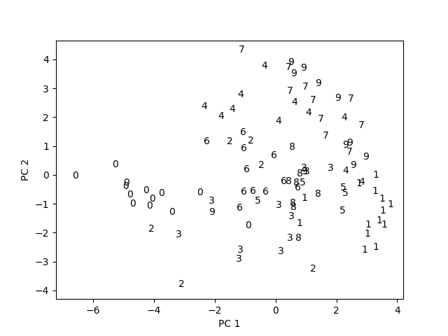
Part 4: first 2 principal components visualization
Below is the visualization of the first 2 pricipal components of 100 training data points.
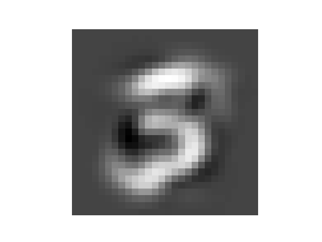
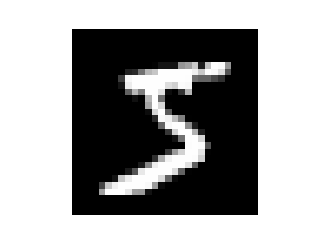
Part 5: image reconstruction from PCA-representations
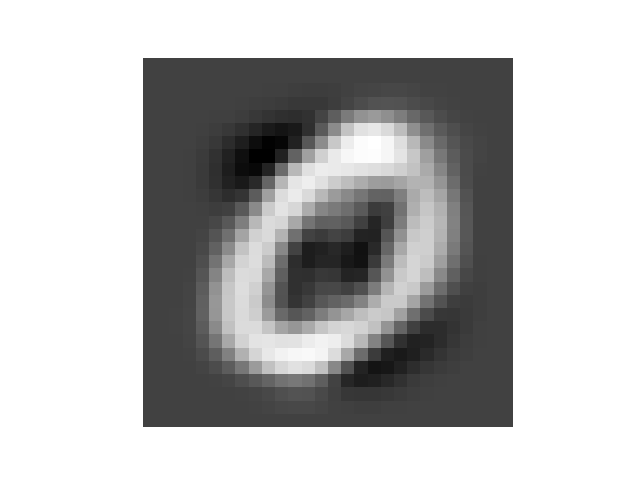
Below are the reconstructions of the first two MNIST images fron their 18-dimensional PCA-representations alongside the originals.
MNIST 1st Image (left: reconstructed, right: original)
MNIST 2nd Image (left: reconstructed, right: original)
Part 6: explicit cubic feature mapping for 2-dimensional case
For \(x = [x_1, x_2]\) and \(\phi(x)^T \phi(x') = (x^T x' + 1)^3\), we expand and get
\[\phi(x)^T \phi(x') = x_1^3{x_1'}^3 + x_2^3{x_2'}^3 + 3 x_1^2{x_1'}^2 x_2 {x_2'} + 3 x_1{x_1'} x_2^2 {x_2'}^2\] \[+ 3 x_1^2{x_1'}^2 + 3 x_2^2{x_2'}^2 + 6 x_1{x_1'} x_2 {x_2'} + 3 x_1 {x_1'} + 3 x_2{x_2'} + 1\]So the corresponding feature vector is
\[\phi(x) = (x_1^3, x_2^3, \sqrt{3} x_1^2 x_2, \sqrt{3} x_1 x_2^2, \sqrt{3} x_1^2, \sqrt{3} x_2^2, \sqrt{6} x_1 x_2, \sqrt{3} x_1, \sqrt{3} x_1, 1)^T\]Part 7: re-train using cubic feature mapping
For practical reason, we apply the feature mapping to 10-dimensional PCA representation instead of original 784-dimensional data.
With same settings as base-line case (e.g., temperature parameter = 1), the test error = 0.0865.
3. Basic Neural Network
Part 4: improve learning rate
Since currently we have constant learning rate, which is not best when approaching the minimum, one way we can do is to reduce learning rate gradually by expressing it as a function of iterations.
Part 5: too many hidden units
The danger would be overfitting.
Part 6: training and test error evolution against epochs
For training error, it will continue going down with epochs, while for test error, it will first go down and then go up.
Part 7: optimize the number of epochs
One way to do is use portion of training data (maybe 10%) as inner validation data, for each epoch we evaluate the inner validation error, if it starts going up consecutively for say, 10 epochs, we stop the training process.
4. Deep Neural Networks
Part 1: fully-connected neural networks
(a) after 10 epochs, the test accuracy = 0.9172.
(b) My final model architecture (mnist_nnet_fc_improved.py) has 6 hidden layers (each has 512 neurons, activation is ReLU) and 1 output layer (with 10 neurons, activation is softmax). Optimizer is SGD(lr=0.03, momentum=0.65, decay=0.0001). With this architecture, the test accuracy = 0.9842.
Among all the tweaks I’ve tried, increasing the number of hidden layers (from 1 hidden layer to 6), the number of neurons (from 128 to 512), the learning rate (from 0.001 to 0.03, I also modified momentum and decay) help a lot, boosting the test accuracy from 0.9172 to 0.9842.
Changing hidden layer activation from ReLU to tanh doesn’t make too much difference, but switching to signmoid really harms test accuracy. Too high or too low decay in learning rate also can damage the accuracy; I believe current choice of decay of 0.0001 is the sweet spot.
Part 2: Convolutional neural networks
(a) A simplest convolutional neural network was constructed in the following order:
-
A 2D convolutional layer with 32 filters of size 3x3
-
A ReLU activation
-
A max pooling layer with size 2x2
-
A ReLU activation
-
A 2D convolutional layer with 64 filters of size 3x3
-
A ReLU activation
-
A max pooling layer with size 2x2
-
A flatten layer
-
A fully connected layer with 128 neurons
-
A dropout layer with drop probability 0.5
-
A fully connected layer with 10 neurons
-
A softmax activation
The implementation using keras is list below:
model = Sequential()
model.add(Conv2D(filters=32,kernel_size=(3,3),input_shape=(1, X_train.shape[2], X_train.shape[3])))
model.add(Activation("relu"))
model.add(MaxPooling2D(pool_size=(2, 2)))

model.add(Conv2D(filters=64,kernel_size=(3,3)))
model.add(Activation("relu"))
model.add(MaxPooling2D(pool_size=(2, 2)))

model.add(Flatten())
model.add(Dense(units=128))
model.add(Dropout(rate=0.5))
model.add(Dense(units=10))
model.add(Activation("softmax"))
The result is quite encouraging, just one epoch, the test accuracy reaches 0.9810. But it does take longer to finish one epoch (48 secs, while 4 secs for the Part 1 fully-connected neural networks).
To speedup the training time and achieve higher test accuracy, I set up CUDA drivers in a accessible GPU and ran the same ConvNN for 15 epochs. Here’s the training log from GPU:
Using Theano backend.
Using cuDNN version 5110 on context None
Mapped name None to device cuda: Quadro K2200 (0000:03:00.0)
Train on 54000 samples, validate on 6000 samples
Epoch 1/15
54000/54000 [================] - 6s - loss: 0.2062 - acc: 0.9346 - val_loss: 0.0555 - val_acc: 0.9822
Epoch 2/15
54000/54000 [================] - 6s - loss: 0.0771 - acc: 0.9771 - val_loss: 0.0408 - val_acc: 0.9878
Epoch 3/15
54000/54000 [================] - 6s - loss: 0.0577 - acc: 0.9820 - val_loss: 0.0351 - val_acc: 0.9887
......
Epoch 12/15
54000/54000 [================] - 6s - loss: 0.0193 - acc: 0.9934 - val_loss: 0.0346 - val_acc: 0.9912
Epoch 13/15
54000/54000 [================] - 6s - loss: 0.0174 - acc: 0.9944 - val_loss: 0.0317 - val_acc: 0.9912
Epoch 14/15
54000/54000 [================] - 6s - loss: 0.0157 - acc: 0.9945 - val_loss: 0.0345 - val_acc: 0.9912
Epoch 15/15
54000/54000 [================] - 6s - loss: 0.0151 - acc: 0.9948 - val_loss: 0.0348 - val_acc: 0.9905
 8832/10000 [===========>....] - ETA: 0sLoss on test set:0.0324026019065 Accuracy on test set: 0.9902
It achieves 99.02% of test accuracy after 15 epochs, and each epoch takes only 6 secs.
5. Classification for overlapping multi-digit MNIST
Pre-step: data representation and model arguments
Training set has 40,000 examples, each example is 42x28 size image, which has two labels indicating two overlapping digits in the image. Each label is a vector of length 10.
Testing set has 4,000 examples, each example is also 42x28 size image, which also has two labels indicating two overlapping digits in the image. Each label is a vector of length 10.
y_train[0] is the fisrt digits in the training images, while y_train[1] is the second.
For model.compile, loss='categorical_crossentropy' means the loss function type is cross entropy function for both outputs, optimizer='sgd' means algorithm is using stochastic gradient descent method to learn, metrics=['accuracy'] means accuracy is used as metric, and loss_weights=[0.5, 0.5] means the two labels are equally treated when calculating loss.
For model.fit, X_train, [y_train[0], y_train[1]] are the training data and their labels, epochs=nb_epoch means total epochs for training, batch_size=batch_size means training is using mini-batch gradient descent approach, and verbose=1 is setting the logging verbosity.
Five explored models
model1: mlp (coded in mlp.py)
The architecture is shown below, with one hidden layer of 64 neurons (relu activation).
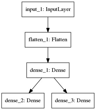
After training 30 epochs, the test accuracy for 1st label is 0.9378, for 2nd label is 0.9278.
Total training time is 3 secs/epoch, total 90 secs (run on NVIDIA Quadro K2200 GPU, same for all the other four models).
model2: mlp2 (coded in mlp2.py)
The architecture is shown below, with 6 hidden layer of 64 neurons (relu activation).
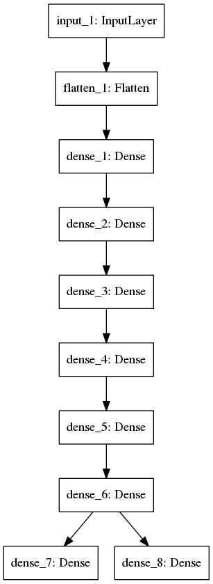
After training 30 epochs, the test accuracy for 1st label is 0.9503, for 2nd label is 0.9429.
Total training time is 4 secs/epoch, total 120 secs.
model3: conv (coded in conv.py)
The architecture is shown below. The first Conv2D has 8 filters, and second has 16 filters. SGD is the optimizer.
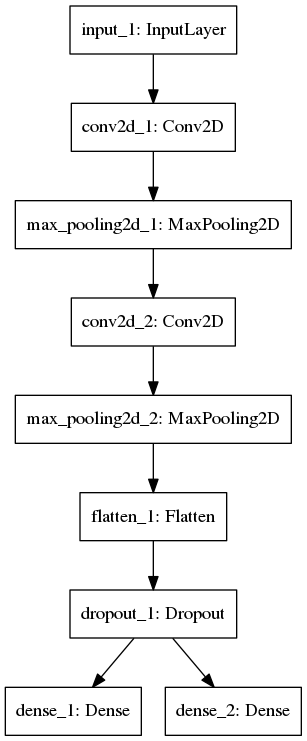
After training 15 epochs, the test accuracy for 1st label is 0.9828, for 2nd label is 0.9755.
Total training time is 14 secs/epoch, total 210 secs.
model4: conv2 (coded in conv2.py)
The architecture is exactly same as model conv. The difference is adam is the optimizer.
After training 15 epochs, the test accuracy for 1st label is 0.9869, for 2nd label is 0.9822.
Total training time is 14 secs/epoch, total 210 secs.
model5: conv3 (coded in conv3.py)
The architecture is exactly same as model conv. The difference is that the first Conv2D has 32 filters, and second has 64 filters
After training 15 epochs, the test accuracy for 1st label is 0.9890, for 2nd label is 0.9869.
Total training time is 39 secs/epoch, total 585 secs.
Thoughts on model selection
It seems that convolutional neural networks are more effective in learning images than fully connected neural networks. Model mlp and mlp2 can only achieve test accuracy around 0.95, while conv, conv2 and conv3 can easily achieve beyond 0.98.
For fully connected neural networks, adding more hidden layers seems helpful at least from 1 hidden layer to 6 hidden layers.
Sometime optimizer can make a difference as well, e.g., here using adam optimizer is more effective than SGD to reach minimum.